Why EBaMl?
An EBM is a glass-box model: a person can read every part of it. But a model with many features has many graphs, and each graph can have hundreds of bins. A customer who asks "why was my loan denied?" does not want a graph. EBaMl puts the graphs and the predictions of an EBM into words, and it computes in Python every fact that the words state.
This page follows one model from the graph to the words. The model is an EBM of synthetic loan data, with the features
income, debt_ratio, age and late_payments. The docs build fits it and computes the graph, the graph text and
the facts below (scripts/docs/figures.py). The texts in the boxes marked "Example" come from one run of an LLM. Another
run, or another model, gives other words.
From a graph to a description
interpret shows the graph of a feature as a picture:
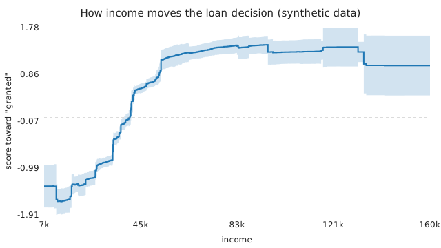
Many LLMs read only text. A vision model can read the picture, but it estimates each value from the axes. So EBaMl
writes the graph as text, which every model reads and which gives the exact numbers. EBMGraph.to_text lists the
score and the confidence interval of each bin. The text below drops the bins that change the score by less than 5 % of its range
(EBMGraph.simplify):
This graph represents a continuous-valued feature. The keys are intervals that represent ranges where the function predicts the same value.

Feature Name: income
Feature Type: continuous
Means: {"(6900.0, 11700.0)": -1.341, "(11700.0, 17750.0)": -1.605, "(17750.0, 24750.0)": -1.349, "(24750.0, 27250.0)": -1.193, "(27250.0, 30150.0)": -1.037, "(30150.0, 34050.0)": -0.882, "(34050.0, 34250.0)": -0.662, "(34250.0, 37050.0)": -0.438, "(37050.0, 37750.0)": -0.283, "(37750.0, 40850.0)": -0.128, "(40850.0, 41350.0)": 0.03, "(41350.0, 42050.0)": 0.27, "(42050.0, 45950.0)": 0.439, "(45950.0, 50850.0)": 0.594, "(50850.0, 52850.0)": 0.755, "(52850.0, 53150.0)": 0.924, "(53150.0, 67450.0)": 1.141, "(67450.0, 133300.0)": 1.297, "(133300.0, 159500.0)": 1.06}
Lower Bounds (95%-Confidence Interval): {"(6900.0, 11700.0)": -1.779, "(11700.0, 17750.0)": -1.907, "(17750.0, 24750.0)": -1.586, "(24750.0, 27250.0)": -1.366, "(27250.0, 30150.0)": -1.222, "(30150.0, 34050.0)": -0.996, "(34050.0, 34250.0)": -0.899, "(34250.0, 37050.0)": -0.587, "(37050.0, 37750.0)": -0.426, "(37750.0, 40850.0)": -0.289, "(40850.0, 41350.0)": -0.198, "(41350.0, 42050.0)": 0.005, "(42050.0, 45950.0)": 0.271, "(45950.0, 50850.0)": 0.489, "(50850.0, 52850.0)": 0.562, "(52850.0, 53150.0)": 0.715, "(53150.0, 67450.0)": 0.927, "(67450.0, 133300.0)": 0.913, "(133300.0, 159500.0)": 0.472}
Upper Bounds (95%-Confidence Interval): {"(6900.0, 11700.0)": -0.903, "(11700.0, 17750.0)": -1.303, "(17750.0, 24750.0)": -1.112, "(24750.0, 27250.0)": -1.02, "(27250.0, 30150.0)": -0.852, "(30150.0, 34050.0)": -0.767, "(34050.0, 34250.0)": -0.426, "(34250.0, 37050.0)": -0.29, "(37050.0, 37750.0)": -0.14, "(37750.0, 40850.0)": 0.034, "(40850.0, 41350.0)": 0.259, "(41350.0, 42050.0)": 0.534, "(42050.0, 45950.0)": 0.606, "(45950.0, 50850.0)": 0.698, "(50850.0, 52850.0)": 0.949, "(52850.0, 53150.0)": 1.134, "(53150.0, 67450.0)": 1.356, "(67450.0, 133300.0)": 1.68, "(133300.0, 159500.0)": 1.647}
describe_graph sends this text to the LLM in a chain of three turns, and returns a description of the graph:
Example: the description of the graph of income (one run of openrouter/free)
The income function shows a strong overall increase from approximately –1.6 at the lowest earnings to positive values, crossing zero near $40,000–$41,000 and indicating that lower incomes substantially hinder loan approval while higher incomes generally help. Between roughly $55,000 and $95,000 the curve plateaus at a high positive level of about +1.3 to +1.4, reflecting a strong and fairly stable benefit from moderate-to-high income. The most striking feature is what occurs above $95,000, where the function unexpectedly declines, dropping to around +1.29 for incomes between $95,400 and $116,500 and further to about +1.03 in the top bin $133,300–$159,500, which contradicts the intuitive expectation that more income always strengthens approval odds. This decline coincides with very wide confidence intervals, especially in the highest bins, suggesting the pattern is driven by sparse data rather than a robust real effect. [...]
describe_ebm describes each graph in the same way, and then writes a summary of the whole model.
From a prediction to an explanation
A local explanation explains one prediction. Take this applicant, whom the model denies:
{
  "income": 31500.0,
  "debt_ratio": 0.46,
  "age": 67.0,
  "late_payments": 1.0
}
interpret gives the contribution of each feature to this prediction. EBaMl answers three questions that a person
asks (Barceló et al., 2020): what must change to flip the decision, which inputs settle the decision on their own, and
how certain the decision becomes as the inputs become known. Python computes the answers from the scores and the
confidence intervals of the EBM. For a data scientist, the facts of the first two questions are:
{
  "flip_possible": true,
  "changes": [
    {
      "feature": "income",
      "from": "3.15e+04",
      "to": "[8.29e+04, 8.315e+04)",
      "score_change": 2.292
    }
  ],
  "number_of_changes": 1,
  "is_smallest_set": true,
  "smallest_possible_number_of_changes": 1,
  "after_the_changes": {
    "predicted_class": "granted",
    "probability": 0.614
  },
  "flip_holds_at_confidence": 0.95,
  "rare_values_left_out": true,
  "min_support": 0.01
}
{
  "exists": true,
  "features": [
    "income",
    "debt_ratio"
  ],
  "is_smallest_set": true,
  "smallest_possible_number_of_features": 2,
  "features_not_needed": [
    "late_payments",
    "age"
  ],
  "guaranteed_margin_logit": 0.612,
  "guarantee_holds_at_confidence": 0.95,
  "rare_values_left_out": true,
  "min_support": 0.01
}
is_smallest_set says that no smaller set of features works. The proof of the local
explanations shows this for the search of the code. The LLM only puts the facts into words.
For a layperson, the facts have no scores, and the probabilities become words:
Example: the explanation for a layperson (one run of openrouter/free)
What would change the decision. The prediction is "denied," and it is very likely, mainly because an income of $31,500 and a debt ratio of 0.46 each push strongly toward denial, one late payment adds a moderate push, and age 67 pushes slightly the other way. To get a different answer, only one thing has to change: income would need to rise from $31,500 into the range from $82,900 up to just under $83,150. That is the smallest change that works — nothing smaller flips the outcome, and no adjustment to the debt ratio, late payments, or age is needed. [...]
What settles the decision. This model's prediction of "denied" is already settled by just two inputs: the applicant's income of $31,500 and debt ratio of 0.46. The other two inputs — one late payment and age 67 — cannot change this outcome for any realistic values they might take, because rare extreme values are excluded from the guarantee. [...] This statement describes how this particular model behaves, not what would happen in the real world.
The result of explain_instance holds the facts next to the words (explanation.facts), so a person can check each
sentence. The words of an LLM can still be wrong. Local explanations says what each
guarantee means and what it does not mean.
To compute the facts alone, with no LLM and no API key, call compute_local_facts:
from interpret.glassbox import ExplainableBoostingClassifier

from ebaml import DataScientist, compute_local_facts, facts_to_texts

ebm = ExplainableBoostingClassifier(interactions=0).fit(X, y)
facts = compute_local_facts(ebm, X.iloc[0].to_dict())
print(facts_to_texts(facts, DataScientist()).counterfactual)  # the JSON that the LLM reads
What EBaMl adds to interpret
| Task | interpret |
EBaMl |
|---|---|---|
| Read a graph | A picture of the graph. | The graph as text, and a description of the graph in words (describe_graph). |
| Read the whole model | One picture for each graph, and the importance of each feature. | A summary of the model in words (describe_ebm). |
| Explain one prediction | The contribution of each feature. | A counterfactual, a sufficient reason and completions, computed in Python and put in words for a layperson or a data scientist (explain_instance). |
| Change the model | Methods of the model for whole terms: monotonize, scale, remove_terms. |
Edits of single bins and ranges of a graph, as in GAM Changer, with a report, a history and business constraints (EditSession). See Editing a model. |
| Give the model to an agent | No tool for agents. | An MCP server with tools to read, explain and edit the model (ebaml-mcp). See MCP server. |
| Choose the LLM | Not applicable. | Any provider from Python with model=: OpenRouter, OpenAI, Anthropic, Gemini, Ollama and more. See Choosing the model. |
EBaMl is based on TalkToEBM (Lengerich et al., 2023), which showed that an LLM can read the graph text of an EBM. The home page says how the two differ.
Next steps
- Install EBaMl and set an API key: Setup.
- Describe a graph and a model: Usage.
- Explain one prediction: Local explanations.
References
- Barceló, P., Monet, M., Pérez, J. and Subercaseaux, B. (2020). Model Interpretability through the Lens of Computational Complexity. NeurIPS 2020. arXiv:2010.12265.
- Lengerich, B. J., Bordt, S., Nori, H., Nunnally, M. E., Aphinyanaphongs, Y., Kellis, M. and Caruana, R. (2023). LLMs Understand Glass-Box Models, Discover Surprises, and Suggest Repairs. arXiv:2308.01157.